Reducing Colors In An Image ⇢ Dithering

Introduction

An image can be rendered on a computer screen using millions of colors. In a traditional bitmap, every pixel is represented by a RGB value — the red, green, and blue channels. The value of each color can vary between 0-255. This means there are over 16 million (256 * 256 * 256 = 16,777,216) possible colors!

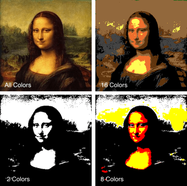
What if you did not have millions of colors at your disposal? Think about older devices, printers (both 2D and 3D), or printing presses making giant posters of your favorite movie. You may also want to reduce your color palette to reduce the memory usage.

What you need is some sort of mapping, that maps the pixel with 16 million possible colors, to say 8 possible colors. Intuitively, the best approach would be to figure out which of the 8 colors is most similar to the pixel's color and use this similarity for mapping.

Finding the closest color

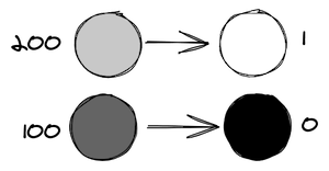
Let's start with a simple case - a binary image where each pixel is either black or white. In a grayscale image each pixel can have a value between 0-255. For a binary image, if the value is closer to white (>=128), use white, else black.

You can play the same game with colors. Imagine the r,g,b colors as values along the axes in 3D cartesian coordinates. 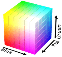Color similarity can be measured as the distance between two points (r1, g1, b1) and (r2, g2, b2) in 3D cartesian space.

d = sqrt((r2-r1)² + (g2-g1)² + (b2-b1)²)

Humans, though, do not perceive the red, green, and blue shades the same way. So colors are usually weighted to better match human vision — red 30%, green 59%, and blue 11%. Better yet, use the CIELAB color space, which describes a color closer to how humans perceive color.

ΔE = sqrt(ΔL² + Δa² + Δb²)

So the distance in CIELAB space would more accurately depict the closeness of two colors (more on this).

Palette mapping is not enough

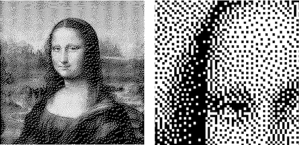
Take a moment to try the interactive demo at the top of this page with dithering OFF. You will notice that the output is not quite as attractive.

A one-to-one mapping of colors does the job, but we lose the character in the image. We can do better, and believe it or not, we do it by adding noise to the image.

Dithering!

When we approximated the colors from one palette to another, the difference in the color introduced in the pixel is called quantization error. Dithering is applying noise to the image to distribute these quantization errors.

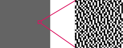
Take a simple example of gray rectangle (grayscale value 100). Mapping the rectangle to binary, every pixel in the rectangle will turn black because 100 is less than 128. But, what if, instead, we turn pixels black or white with such a density that the average gray level is maintained — at least to the human eye when looked at a distance.

Error Diffusion Dithering

Two common ways dithering are Ordered and Error Diffusion. Ordered dithering is based on a fixed matrix and is localized — a pixel's value does not influence the dithering of surrounding pixels. Read more about it here. In Error Diffusion dithering, the quantization error of a pixel is distributed to the surrounding pixels. Unlike Ordered dithering, Error Diffusion can work with any color palette, which is the main reason I'll focus on it.

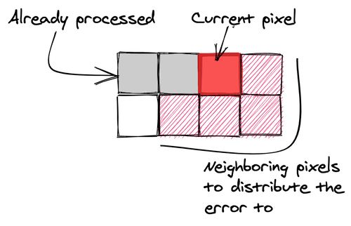
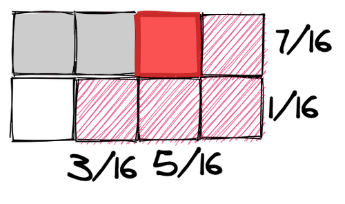
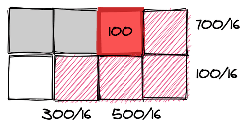
A popular version of Error Diffusion dithering is Floyd–Steinberg dithering. In this algorithm you go through one pixel at time - left to right, and top to bottom. For each pixel, we distribute the quantization error to the surrounding pixels that have not been processed yet. Floyd–Steinberg suggests that the error is distributed in fractions of 7/16, 1/16, 5/16, 3/16 in clockwise directions.

Let's work on an example. Keeping it simple at first, a grayscale image to binary. Let's say the current pixel value is 100, which gets resolved to 0 in binary. The quantization error for the pixel is 100 - 0 = 100. This error is now distributed to the surrounding pixels using the fractions defined above.

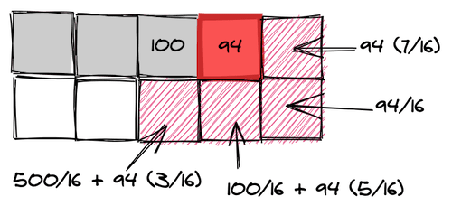
Moving on to the next pixel, the pixel to the right of the previous one. The value of this pixel is, say, 50. It also has the error from the previous pixel, so the effective value of this pixel is 50 + 700/16 ≅ 94. Now 94 also approximates to 0 with a quantization error of 94 which is further distributed to the following pixels.

Dithering with color

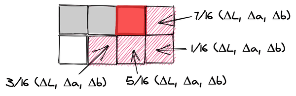
The algorithm can now easily be extrapolated to the CIELAB color space. The quantization error is not a number anymore, but a tuple of individual difference in the LAB colors (ΔL, Δa, Δb). When distributing the error, each value of the tuple is multiplied by the associated fraction.

Note: Since writing this, people have suggested that dithering would work better in RGB space causing less hue shift. Finding the closest color using CIELAB color space but distribute the quantization error in RGB. I tested this and the color boundaries do look better but the image brightness seems to be affected as well. When working with binary images though, certain images created a banding effect around some color boundaries, which did not appear in CIELAB space.

Formalize the algorithm

Floyd–Steinberg dithering explained above can be formalized as follows:

for each y from top to bottom do
    for each x from left to right do
        oldpixel := pixel[x][y]
        newpixel := find_closest_palette_color(oldpixel)
        pixel[x][y] := newpixel
        quant_error := oldpixel - newpixel
        pixel[x + 1][y    ] := pixel[x + 1][y    ] + quant_error × 7 / 16
        pixel[x - 1][y + 1] := pixel[x - 1][y + 1] + quant_error × 3 / 16
        pixel[x    ][y + 1] := pixel[x    ][y + 1] + quant_error × 5 / 16
        pixel[x + 1][y + 1] := pixel[x + 1][y + 1] + quant_error × 1 / 16

Demo it again, good sir!

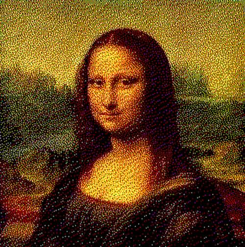
Take a moment to play with this interactive demo of Dithering (Yes, this is the same as the one on top of the post).

How I got here + Epilogue

I was trying to solve a problem where I could map images created by LegraJS to actual available Lego pieces — Figure out what Lego pieces one would need in what color. This led me to image color reduction and then to Dithering. I have since discovered that dithering is not the right solution for that use case... more on that later. But, it was fascinating to discover the process. I was aware of dithering but never got around to actually implementing it. Code for the TypeScript implementation I wrote can be found on the cielab-dither repo.

For the interactive demo on this page, I used this implementation and run the algorithm in a WebWorker. I wrapped the demo as a WebComponent and just drop the element wherever I needed in the blog post: <dither-view></dither-view>

Feel free to reach out to me on Twitter with any feedback or comments. Cheers!